How to Prevent Duplicate Entries in Excel & Google Sheets

This tutorial demonstrates how to prevent duplicate entries in Excel and Google Sheets.

 

 

Prevent Duplicate Entries

If you want to allow only unique values in a column, use the data validation functionality in Excel. This way, you can prevent a user from entering duplicate values. Say you have the following list of names in Column B.

 

 

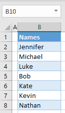
To prevent duplicate entries in a range, follow these steps:

1. Select the range for data validation (e.g., B2:B10), and in the Ribbon, go to Data > Data Validation.

 

 

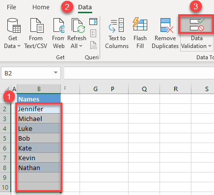
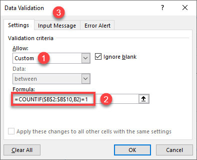
2. In the Data Validation window, (1) select Custom as the validation criteria under Allow, and (2) enter the COUNTIF formula:

=COUNTIF($B$2:$B$10,B2)=1

This formula counts – for each entry – how many times that value appears in the range B2:B10. If the result is 1 (meaning the entry appears only once in the range) then it is allowed. Otherwise, the data validation rule prevents a user from entering that value, since it is already in the range.
Then (3) go to the Input Message tab.

 

 

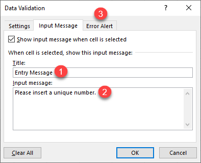
3. In the Input Message tab, enter (1) the Title of the message you’re adding and (2) the Input message. This message appears when a user selects a cell in the data validation range to provide information about the data validation rule.
   Then (3) go to the Error Alert tab.

 

 

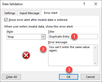
4. In the Error Alert tab, enter (1) the Title of the error message and (2) the Error message. This message appears if a user enters an existing value and prevent them from entering duplicate values.
   Then (3) click OK.

 

 

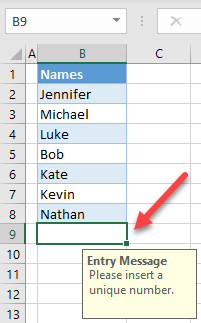
Now selecting an empty cell from the data validation range (for example, B9) prompts an input message about data validation.

 

 

If you try to enter an existing value in cell B9 (e.g., Michael), you get the error message pictured below, stopping you from entering a duplicate value.

 

 

Note: To remove duplicate values or duplicate rows that were already present in the data, see How to Remove Duplicate Cells or this VBA tutorial.

Prevent Duplicate Entries in Google Sheets

To prevent duplicate entries in Google Sheets, follow these steps.

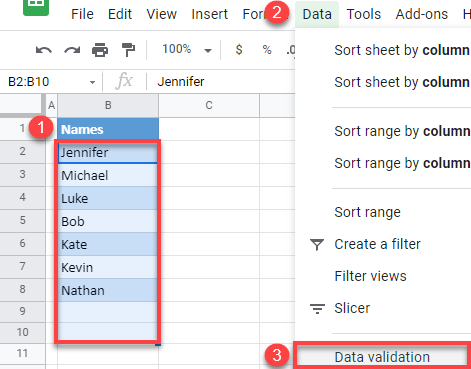
1. Select the range for data validation (e.g., B2:B10), and in the Menu, go to Data > Data validation.

 

 

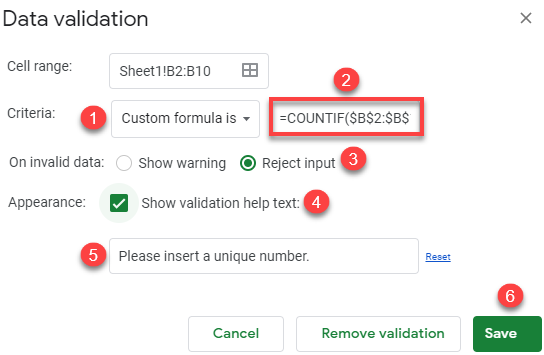
2. In the Data validation window, (1) enter Custom formula is as the Criteria, and (2) enter the formula:

=COUNTIF($B$2:$B$10,B2)=1

Then (3) select Reject input, (4) check Show validation help text, and (5) enter an error message. (6) Click Save.

 

 

Now, if you try to enter a value in cell B9 that already exists in the range, you get the error message you just set.