Data Validation Custom Formulas
This tutorial will demonstrate you how to create custom formulas in Data Validation in Excel and Google Sheets
Data Validation – Must Begin With – Excel
We can write a custom formula to ensure that the data in a cell begins with certain text.

- Highlight the range required eg: B3:B8.
- In the Ribbon, select Data > Data Tools > Data Validation.

- Select Custom from the Allow drop-down box, and then type the following formula:
=EXACT(LEFT(B3,4),”FRU-“)
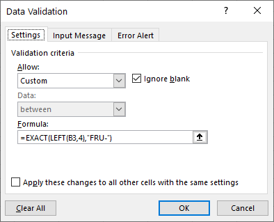
The formula uses 2 functions EXACT and LEFT to determine if the first 4 characters entered into the cell are identical to “FRU-”
- If you want to add an input message for your user, click Input Message.

- Make sure the tick box “Show input message when cell is selected” is checked and then type in the title and message you require.
- If you want to add an error alert, click Error Alert.
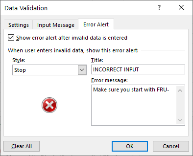
- You can change the Style from Stop to either Warning or Information if you require, and then type in your title and error message.
- Click OK.
- If you have used the Input Message option, a comment will appear on the screen informing the user of the rule.

- Type “FRI-124” in cell B3. If you have selected Stop, the following message box will appear.

- If you selected Warning, then this message box will appear. This allows you to continue if you determine that the data is correct.

- If you have selected Information, then this message box will appear.

- If you click OK, you will be allowed to continue with the incorrect data entered into the cell.
- Click Cancel to exit the message or OK to enter the text into the cell.
Data Validation Allow Uppercase Only in Excel
We can write a custom formula to ensure that the data in a cell only allows upper case if text is entered into the cell.

- Highlight the range required eg: B3:B8.
- In the Ribbon, select Data > Data Tools > Data Validation.
- Select Custom from the Allow drop-down box, and then type the following formula:
=EXACT(B3,UPPER(B3))
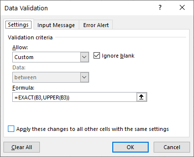
The formula uses 2 functions EXACT and UPPER to determine if the text entered into the cell is in uppercase. Cells with a mixture of number and text are considered text and the numbers are ignored in the rule.
- Click OK.
- Type “fru-124” in cell B3.
- If you have used the Error Alert option, your custom warning and error message will appear. If you have not used this option, the standard warning will appear.

- Click Cancel to exit the message or Retry to re-enter correct text into the cell.
- Type “123456” in cell B3.
- This will be allowed as it is a number and not text.
In our next example, we will ensure that only uppercase text can be entered into the cell.
Data Validation Allow Uppercase Text Only in Excel
We can write a custom formula in Data Validation can be used to ensure that the data in a cell only allows upper case text
NOTE: if you enter information into a cell that begins with text but contains numbers, Excel will consider the information text.
- Highlight the range required eg: B3:B8.
- In the Ribbon, select Data > Data Tools > Data Validation.
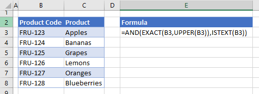
- Select Custom from the Allow drop-down box, and then type the following formula:
=AND(EXACT(B3,UPPER(B3)),ISTEXT(B3))

The formula uses 4 functions AND, EXACT, UPPER and TEXT to determine if the text entered into the cells is in Upper Case AND to determine if the information entered is actually text and not a pure number.
- Click OK.
- Type “fru-124” in cell B3.
- If you have used the Error Alert option, your custom warning and error message will appear. If you have not used this option, the standard warning will appear.

- Click Cancel to exit the message or Retry to re-enter correct text into the cell.
- Type “123456” in cell B3.
- You will once again get the error message.
- Click Cancel to exit the message or Retry to re-enter correct text into the cell.
Data Validation Prevent Spaces in Excel
We can write a custom formula to ensure that no spaces are entered into the data entered in a range of cells.

- Highlight the range required eg: B3:B8.
- In the Ribbon, select Data > Data Tools > Data Validation.
- Select Custom from the Allow drop-down box, and then type the following formula:
=B3=SUBSTITUTE(B3, ” ” , “”)

The formula uses the SUBSTITUTE Function to check that spaces do not exist.
- Click OK.
- Type “FRU – 124” in cell B4.
- If you have used the Error Alert option, your custom warning and error message will appear. If you have not used this option, the standard warning will appear.

- Click Cancel to exit the message or Retry to re-enter correct text into the cell.
Data Validation Prevent Duplicates in Excel
We can write a custom formula to prevent us from entering duplicate information into a range of cells.
- Highlight the range required eg: B3:B8.
- In the Ribbon, select Data > Data Tools > Data Validation.
- Select Customer from the Allow drop-down box, and then type the following formula:
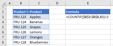
=COUNTIF($B$3:$B$8,B3)<2

The formula uses the COUNTIF Function and uses ABSOLUTES in the range B3:B8 to ensure that this is the list that the COUNTIF Function looks at when it checks to see if there are any duplicate values.
- Click OK.
- Type “FRU-123” in cell D4.
- If you have used the Error Alert option, your custom warning and error message will appear. If you have not used this option, the standard warning will appear.

- Click Cancel to exit the message or Retry to re-enter correct text into the cell.
Data Validation Exists in List in Excel
We can write a custom formula ensure that only specific text is entered into a cell.
- Highlight the range required eg: D3:D8.
- In the Ribbon, select Data > Data Tools > Data Validation.
- Select Custom from the Allow drop-down box, and then type the following formula:
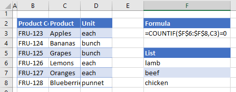
=COUNTIF($F$6:$F$8,D3)>0
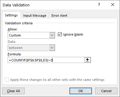
The formula uses the COUNTIF function and uses ABSOLUTES in the range F3:F8 to ensure that this is the list that the COUNTIF function looks at when it checks to see that the correct text is being entered.
- Click OK.
- Type “Single” in cell D4.
- If you have used the Error Alert option, your custom warning and error message will appear. If you have not used this option, the standard warning will appear.

- Click Cancel to exit the message or Retry to re-enter correct text into the cell.
Data Validation Does not Exist in List in Excel
We can use a custom formula ensure that specific text is not entered into a cell.

- Highlight the range required eg: C3:C8.
- In the Ribbon, select Data > Data Tools > Data Validation.
- Select Customer from the Allow drop-down box, and then type the following formula:
=COUNTIF($F$6:$F$8,C3)=0

The formula uses the COUNTIF function and uses ABSOLUTES in the range F3:F8 to ensure that this is the list that the COUNTIF function looks at when it checks to see that the correct text is being entered.
- Click OK.
- Type “Beef” in cell C4.
- If you have used the Error Alert option, your custom warning and error message will appear. If you have not used this option, the standard warning will appear.

- Click Cancel to exit the message or Retry to re-enter correct text into the cell.
Data Validation Only Numbers are Entered in Excel
We can use a custom formula to ensure that only a number is entered into a cell.

- Highlight the range required eg: F3:F8.
- In the Ribbon, select Data > Data Tools > Data Validation.
- Select Customer from the Allow drop-down box, and then type the following formula:
=ISNUMBER(F3:F8)

The formula uses the ISNUMBER function to ensure that a number is entered into the cells in the range.
- Click OK.
- Type “nine” in cell F4.
- If you have used the Error Alert option, your custom warning and error message will appear. If you have not used this option, the standard warning will appear.

- Click Cancel to exit the message or Retry to re-enter correct text into the cell.
Data Validation Does not Exceed Value in Excel
We can use a custom formula ensure that the values entered into a cell do not exceed a specified value.

- Highlight the range required eg: E3:E8.
- In the Ribbon, select Data > Data Tools > Data Validation.
- Select Customer from the Allow drop-down box, and then type the following formula:
=E3<=$G$6

The formula an ABSOLUTE in the range G6 to ensure that this is the value that the rule checks when data is entered into E3.
- Click OK.
- Type “9” in cell E4.
- If you have used the Error Alert option, your custom warning and error message will appear. If you have not used this option, the standard warning will appear.

- Click Cancel to exit the message or Retry to re-enter correct text into the cell.
Data Validation Does not Exceed Total in Excel
We can use a custom formula ensure that the values entered into a range of cells do not exceed a specified total value for the range

- Highlight the range required eg: F3:F8.
- In the Ribbon, select Data > Data Tools > Data Validation.
- Select Customer from the Allow drop-down box, and then type the following formula:
=SUM($F$3:$F$8)<=$H$6
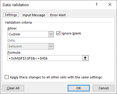
The formula uses the SUM Function and uses ABSOLUTES in the range F3:F8 to ensure that this is the list that the SUM Function looks at when it checks to see that the total of the range is not greater than the value entered in H6.
- Click OK.
- Type “40” in cell F4.
- If you have used the Error Alert option, your custom warning and error message will appear. If you have not used this option, the standard warning will appear.

- Click Cancel to exit the message or Retry to re-enter correct text into the cell.
Data Validation Weekday Dates Only in Excel.
We can use a custom formula to ensure that only weekdays are entered when dates are used in Excel.

- Highlight the range required eg: G3:G8.
- In the Ribbon, select Data > Data Tools > Data Validation.
- Select Customer from the Allow drop-down box, and then type the following formula:
=WEEKDAY(F3,2)<6

The weekday function checks to make sure that the day contained within the date is not a Saturday or a Sunday.
- Amend the date in G5 to show a Saturday (eg 9th May 2020).
- If you have used the Error Alert option, your custom warning and error message will appear. If you have not used this option, the standard warning will appear.
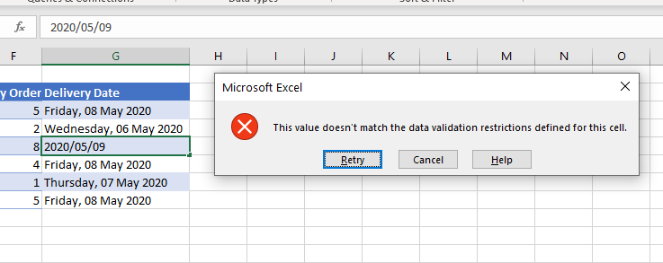
- Click Cancel or Retry to enter an alternative date.
Data Validation Future Date Only in Excel
We can create a custom formula to only allow the user to enter a date that is in the future.

- Highlight the range required eg: G3:G8.
- In the Ribbon, select Data > Data Tools > Data Validation.
- Select Customer from the Allow drop-down box, and then type the following formula:
=G3>TODAY()

The formula uses the TODAY Function to check if the date entered into the cell is greater than today’s date.
- Amend the date in G5 to yesterday.
- If you have used the Error Alert option, your custom warning and error message will appear. If you have not used this option, the standard warning will appear.

- Click Cancel or Retry to enter an alternative date.
Data Validation Must Begin With in Google Sheets

- Highlight the range required eg: B3:B8.
- In the Menu, select Data > Data Validation.

- The cell range will already be filled in.

- Select Custom Formula is from the Criteria drop down list.

- Type in the formula.
=EXACT(LEFT(B3,4),”FRU-“)

- Select either Show Warning or Reject Input if the data is invalid.
![]()
- You can type in some Validation help text if you require.

- Click Save.

- Click in B3 to see the Validation help text

- Type FRI-123
- If you have selected Show Warning, the following message will appear.

- Alternatively, if you have selected Reject Input on Invalid Data, you will be prevented from entering the data and the following message appears on the screen.

The rest of the custom formula examples in Google Sheets work in exactly the same way.