How to Refresh a Pivot Table in Excel
This article will demonstrate how to refresh a pivot table in Excel.
Refresh a Pivot Table
PivotTable Analyze Tab
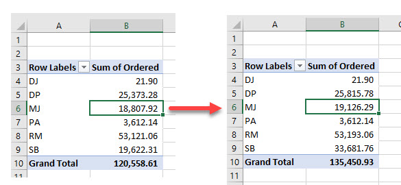
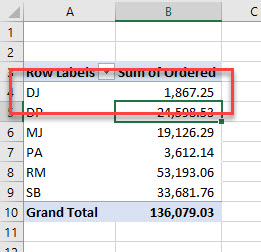
Consider the following pivot table.
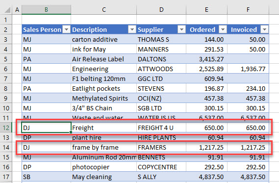
Say you go back to your database and make some adjustments.
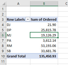
If you switch back to the pivot table, it won’t have changed. To update the pivot table, refresh the data.
- Click in your pivot table.
- Then, in the Ribbon, select PivotTable Analyze > Refresh.
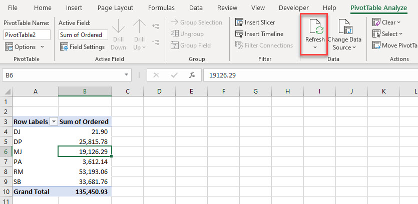
This will refresh the pivot table to include the updated figures.
Refresh With the Quick Menu
- Right-click anywhere inside your pivot table to obtain the Quick Menu.
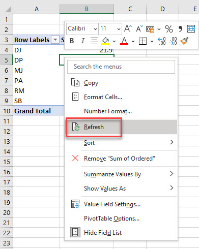
- Select Refresh.
Change the Data Source
If you add any more rows or columns to the range that is selected as the data source, you need to update the data source to reflect these changes. Say, for example, the original range for your pivot table is B2:E81, but then you add more rows to the data.

You would now need to change the data source of your pivot table to include these rows.
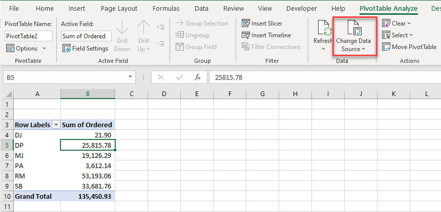
- Click within your Pivot table in order to show the PivotTable Analyze tab in the Ribbon.
- In the Ribbon, select PivotTable Analyze > Data > Change Data Source.
- Amend the range to include your additional rows.
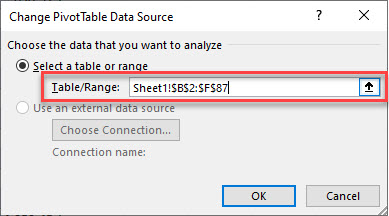
- Click OK to refresh the pivot table.
Refresh All
If you have more than one pivot table or any other linked data in your workbook, you can refresh all the data with one click!
In the Ribbon, select PivotTable Analyze > Data > Refresh > Refresh all.
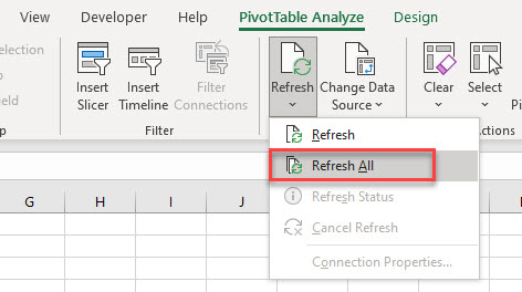
This works for any changes made as long as none of the data ranges have been extended.