Find Duplicates with VLOOKUP or MATCH in Excel & Google Sheets
Download the example workbook
This tutorial will demonstrate how to find duplicate values using VLOOKUP and Match in Excel and Google Sheets. If your version of Excel allows it, we recommend using the XLOOKUP Function to handle duplicates instead.

Find Duplicate Values – VLOOKUP Function
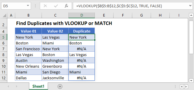
To identify duplicate values in 2 columns in a range of cells in Excel you can use the VLOOKUP Function:
=VLOOKUP($B$4:B$14,$C$4:$C$14, TRUE, FALSE)
If the cities are found in both columns B and C, then they will show in column D.
Find Duplicate Values – MATCH Function
Similarly, you can also find duplicate values in 2 columns using the MATCH Function.
=MATCH(B4,$C$4:$C$14,FALSE)
The MATCH Function will return the row number if the duplicate exists, and a #N/A if the value is not duplicated.
Return Duplicate Value – the IF Function
If you want to return the duplicate value instead of the row number, you can expand the formula created by the MATCH Function to include an IF Function.
Select D4 and type the following formula.
=IF(MATCH(B4,$C$4:$C$14,FALSE)>0,B4,"")
This will give us the exact same result as using the VLOOKUP to return the duplicate value.
Additional Tutorials on Duplicates
Find Duplicate Values in Google Sheets
VLOOKUP Function
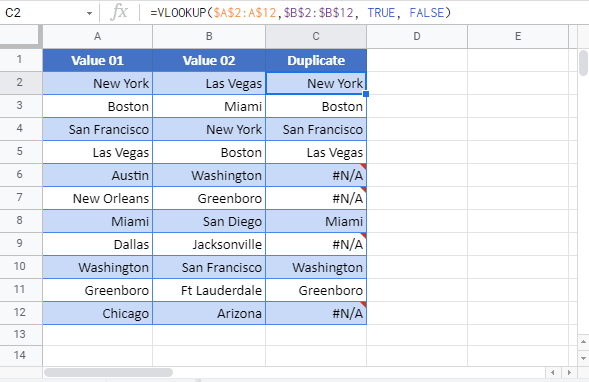
Finding duplicate values in 2 columns using VLOOKUP works exactly the same in Google sheets as it does in Excel.
=VLOOKUP($A$2:A$11,$B$2:$B$12, TRUE, FALSE)
Find Duplicate Values in 2 columns – MATCH Function in Google Sheets
The Match function in Google Sheets is also identical to Excel.
=MATCH(A2,$B$2:$B$12,FALSE)
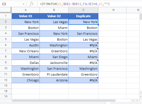
You can also use the IF Function to return the duplicate value.
=IF(MATCH(A2,$B$2:$B$12,FALSE)>0,A2,"")