How To Filter Duplicate Values in Excel & Google Sheets
This tutorial will demonstrate how to filter duplicate values in Excel and Google Sheets.
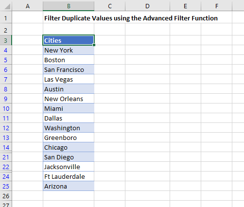
Advanced Filter Function
- Click in the range you wish to apply the filter to (any cell from B3 to B25).
- In the Ribbon, select Data > Sort & Filter > Advanced.

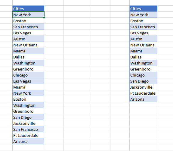
- You can either filter the list in place, or you can put the results in a different range on your worksheet.

- Make sure the check box Unique records only is ticked, and then click OK.
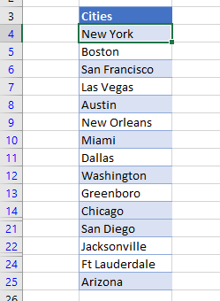
- The rows with duplicate values will be hidden – you will notice that the row numbers are now in blue and some of the rows do not appear.
- In the Ribbon, select Data > Sort & Filter > Clear to remove the filter.

Filter Duplicate Values to an Alternative Range
- Select the range you wish to filter (ex B4:B25).
- In the Ribbon, select Data > Sort & Filter > Advanced.
- Select Copy to another location.
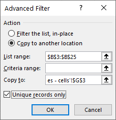
- Select the Range in the Copy to: box and make sure the Unique records only tick box is ticked.
Filter Duplicates Rows using the Advanced Filter Function
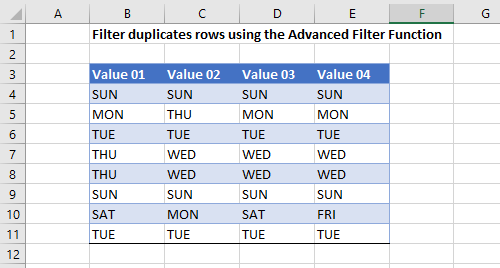
- Click in the range you wish to apply the filter to (any cell from B3 to E11).
- In the Ribbon, select Data > Sort & Filter > Advanced.
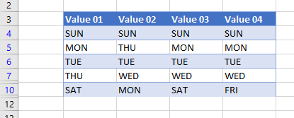
- Filter the list in place and tick the option to show unique records only.
- Click OK.
COUNTIF and the Filter Function in Excel
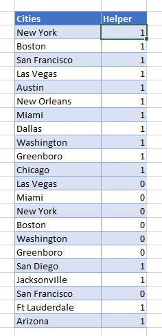
To filter using COUNTIF and standard Filter function, you need to add an additional helper column to your worksheet.
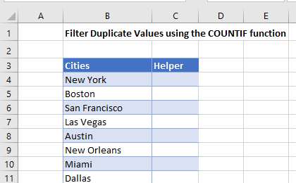
- Click in C4 and type the following formula.
=IF(COUNTIF($B$4:B4,B4)=1,1,0)- Copy it down to row 25.
- If the city appears more than once, a zero will appear next to it when it appears for the second or subsequent time.
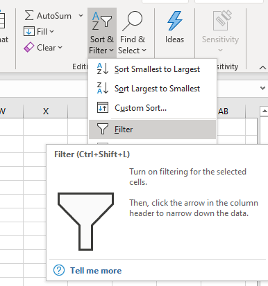
- In the Ribbon, select Home > Filter.
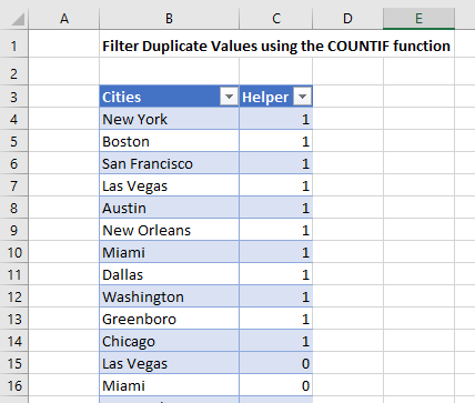
- Dropdown arrows will now appear in the heading row of your list.
- Click the drop-down arrow in the Helper column and select 1 as the value to show.
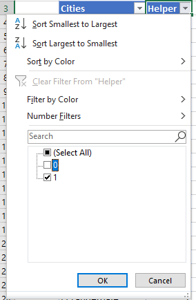
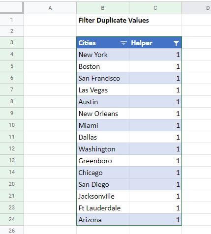
Your list will now be filtered to only show unique values.

COUNTIF and the Filter Function in Google Sheets
Google Sheets does not have an advanced filter feature. You can filter duplicate values by using the same formula as you would use in Excel.
- Click in C4 and type the following formula
=IF(COUNTIF($B$4:B4,B4)=1,1,0)- Copy the formula down to row 25.
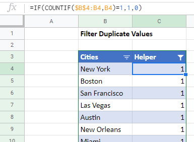
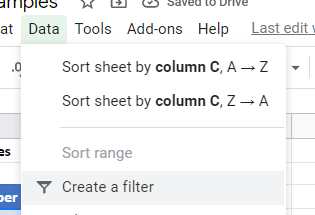
- Select Data>Create Filter from the Menu
- Remove the tick from the 0 so that you are only going to filter on the 1’s.

Click OK to filter the list.
