Find a Number in a Column / Workbook – Excel & Google Sheets

This tutorial will demonstrate how to find a number in a column or workbook in Excel and Google Sheets.

 

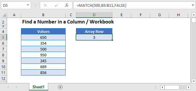
Find a Number in a Column

The MATCH Function is useful when you want to find a number within a array of values.

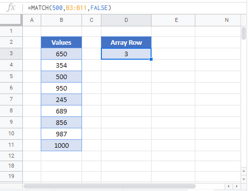
This example will find 500 in column B.

=MATCH(500,B3:B11, 0)

The position of 500 is the 3rd value in the range and returns 3.

Find Row Number of Value Using ROW, INDEX and MATCH Functions

To find the row number of the value found, we can add the ROW and INDEX functions to the MATCH Function.

=ROW(INDEX(B3:B11,MATCH(987,B3:B11,0)))

ROW and INDEX Functions

The MATCH Function returns 3 as we have seen from the previous example. The INDEX Function will then return the cell reference or value of the array position returned by the MATCH Function. The ROW function will then return the row of that cell reference.

Filter in Excel

We can find a specific number in an array of data by using a Filter in Excel.

 

1. Click in the Range you want to filter ex B3:B10.
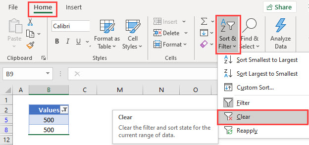
2. In the Ribbon, select Home > Editing > Sort & Filter > Filter.

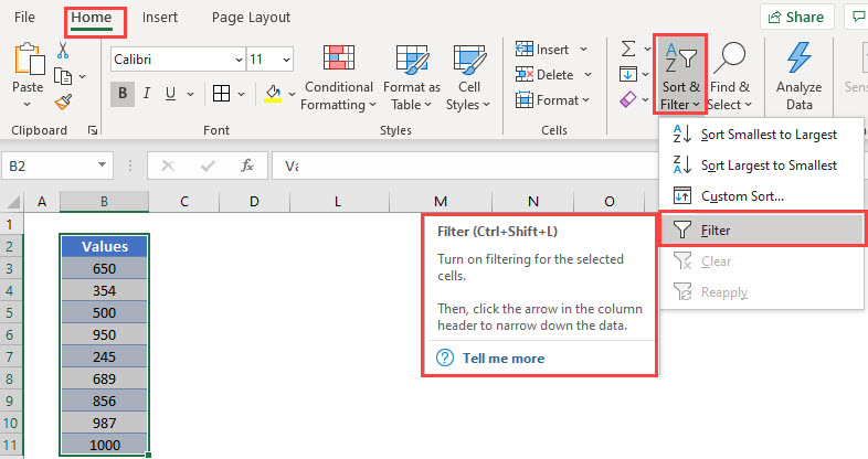
3. A drop-down list will be added to the first row in your selected range.

4. Click on the drop-down list to get a list of available options.

5. Type 500 in the search bar.

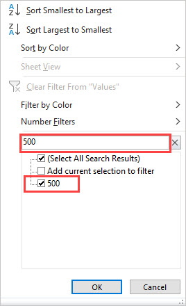
6. Click OK.

7. If your range has more than one value of 500, then both would show.

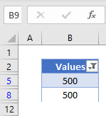
8. The rows that do not contain the required values are hidden, and the visible row headers are shown in BLUE.
9. To clear the filter, click on the drop-down and then click Clear Filter From “Values”.

To remove the filter entirely from the Range, select Home > Editing > Sort & Filter > Clear in the Ribbon.

Find Number in Workbook or Worksheet using FIND in Excel

We can look for values in Excel using the FIND functionality.

1. In your workbook, press Ctrl+F on the keyboard.

OR

In the Ribbon, select Home > Editing > Find & Select.

2. Type in the value you wish to find.

 

3. Click Find Next.

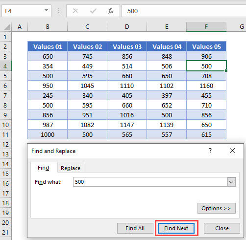
4. Continue to click Find Next to move through all the available values in the Worksheet.
5. Click Find All to find all the instances of the value in the worksheet.

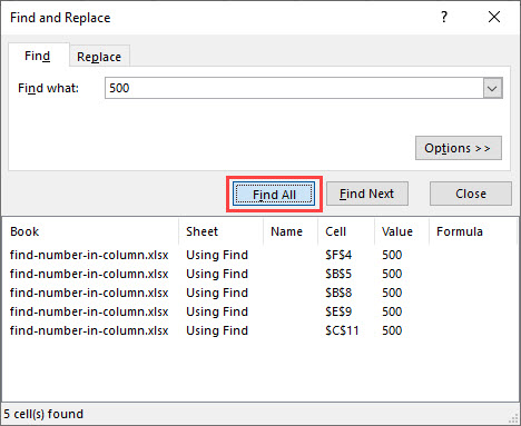
Click Options.

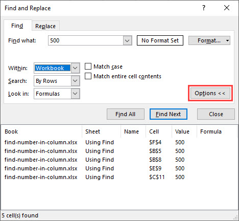
6. Amend the Within from Sheet to Workbook and click Find All

7. All the matching values will appear in the results shown.

 

Find a Number – MATCH Function in Google Sheets

The MATCH Function works the same in Google Sheets as it does in Excel.

Find Row Number of Value Using ROW, INDEX and MATCH Functions in Google Sheets

The ROW, INDEX and MATCH Functions works the same in Google Sheets as it does in Excel.

Filter in Google Sheets

We can find a specific number in an array of data by using Filter in Google Sheets.

1. Click in the Range you want to filter ex B3:B10.
2. In the Menu, select Data > Create a filter

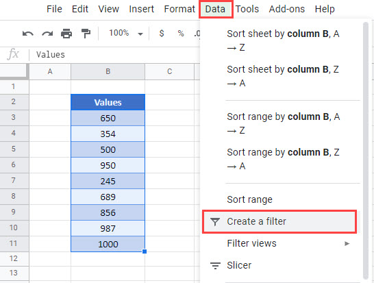
3. In the Search bar, type in the value you wish to filter on.

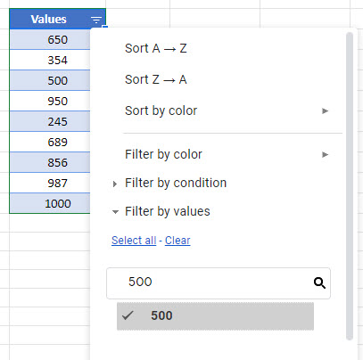
4. Click OK.

5. If your range has more than one value of 500, then both would show.
6. The rows that do not contain the required values are hidden.
7. To clear the filter, click on the drop-down, click Select All” and then click

To remove the filter entire, in the Menu, select Data > Turn off Filter.

 

 

Find Number in Workbook or Worksheet using FIND in Google Sheets

We can look for values in Google Sheets using the FIND functionality.

1. In your workbook, press Ctrl+F on the keyboard.

2. Type in the value you wish to find.
3. All the matching values in the current sheet will be highlighted, with the first one being selected as shown below.

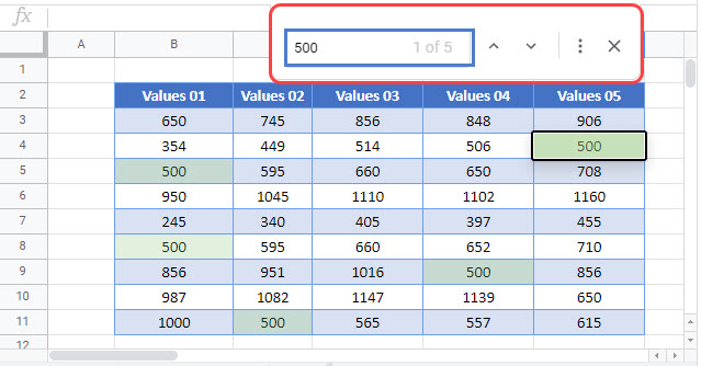
4. Select More Options.

5. Amend the search to All Sheets.

6. Click Find.
7. The first instance of the value will be found. Click Find again to go to the next value and continue to click Find to find all the matching values in the workbook.
8. Click Done to exit out of the Find and Replace Dialog Box.