How to Make Graph Paper in Excel

In this tutorial, you will learn how to make graph paper in Excel.

 

 

If you wish to print graph paper from Excel, adjust cell width and height and change print margins.

Adjust the Size of All Cells

The first step is to change the dimension of cells in the worksheet. To adjust the height of all cells:

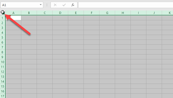
1. Select all cells in the worksheet; click on the arrow in the upper right corner of the worksheet.

 

 

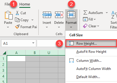
2. Now, in the Ribbon, go to Home > Format and choose Row Height…

 

 

3. In the pop-up window, enter a Row height of 9 and click OK.

 

 

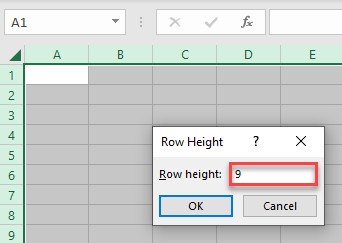
Now the height of all cells in the current worksheet is set to 9. Next, adjust the width of all cells.

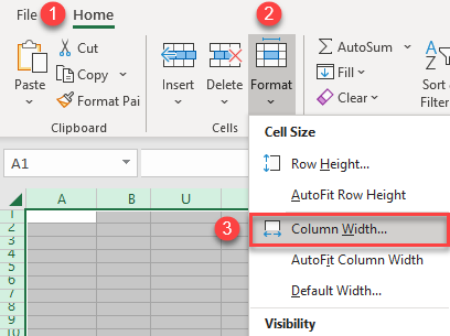
4. Again, select all cells in the worksheet, and then in the Ribbon, go to Home > Format and choose Column Width…

 

 

5. In the pop-up window, enter 1 and click OK.

 

 

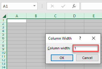
As a result, all cells have the same width and height. To proceed to print, set up the page layout.

Page Setup: Margins and Gridlines

First, change the margins of the document. Here are the steps to follow:

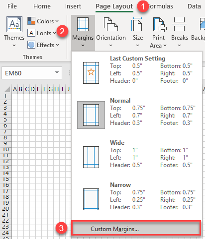
1. In the Ribbon, go to Page Layout > Margins and choose Custom Margins…

 

 

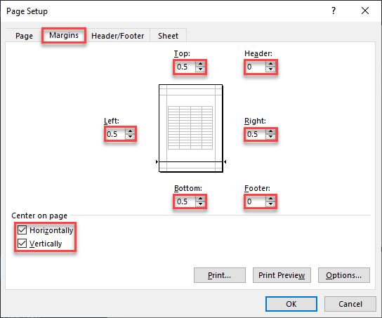
2. The pop-up for Page Setup will appear on the Margins tab. Here, set Top, Left, Bottom, and Right to 0.5 and Header and Footer to 0. Also, check Horizontally and Vertically under Center on page.

 

 

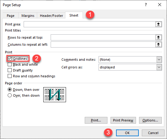
3. After this, go to the Sheet tab, and under Print, check Gridlines. Now we’ve enabled the printing of gridlines, which is necessary for printing graph paper.

 

 

Print Graph Paper

After making all the above changes, you can print the document. Here are the steps for printing:

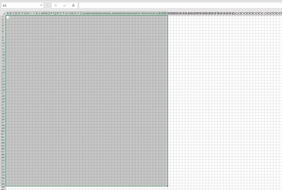
1. Select a page range in the worksheet for printing.

 

 

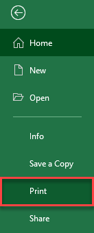
2. In the Ribbon, go to File > Print.

 

 

3. Under Settings, in the first option, instead of default Print Active Sheets, choose Print Selection. This will print just the selection made in the worksheet.

 

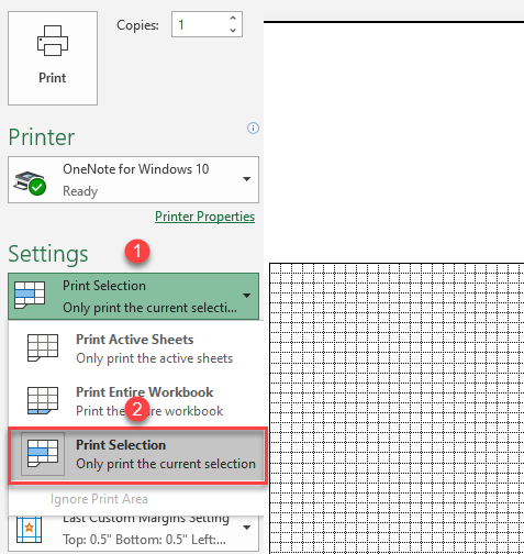
The result is a sheet of graph paper available for printing in Excel, as you can see in the print preview.