How to Select Every Other Row in Excel & Google Sheets
This tutorial demonstrates how to select every other row in Excel and Google Sheets.
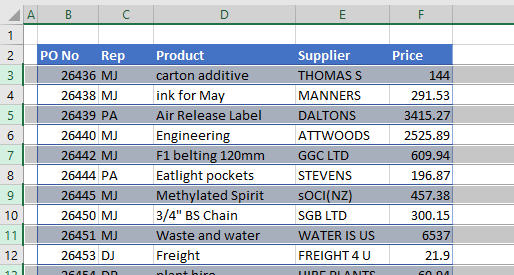
When you’re working with data in Excel, you have a need to select the data in every other row. There are a few ways to select every other row.
Select Every Other Row
Keyboard and Mouse
- Click on the row header to select the first row.

- Holding down the CTRL key on the keyboard, click in the row header of the second row.

- With the CTRL key still held down, click on every other row header until all the rows you need are selected.

Cell Format and Filter
You can use Format as Table and filtering to select every other row.
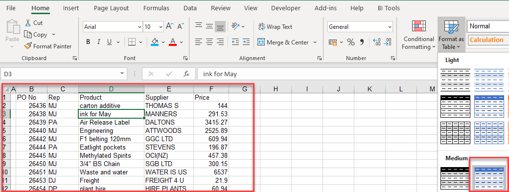
- Highlight the cells whose rows you wish to select. In the Ribbon, go to Home > Cells > Format as Table and select the formatting.
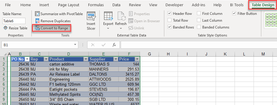
- Then, to remove the table, in the Ribbon, select Table > Convert to Range.
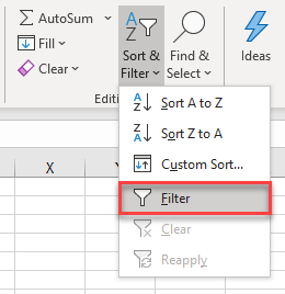
- Next, in the Ribbon, select Home > Editing > Sort & Filter > Filter.
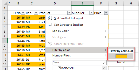
- Click the drop-down arrow on any of the column headings and select Filter by Color.

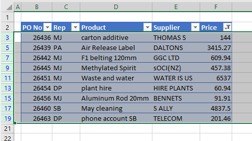
- Every second row is now filtered for. Select these rows.
Conditional Formatting and Filter
You can use Conditional Formatting and Filtering to select every other row.
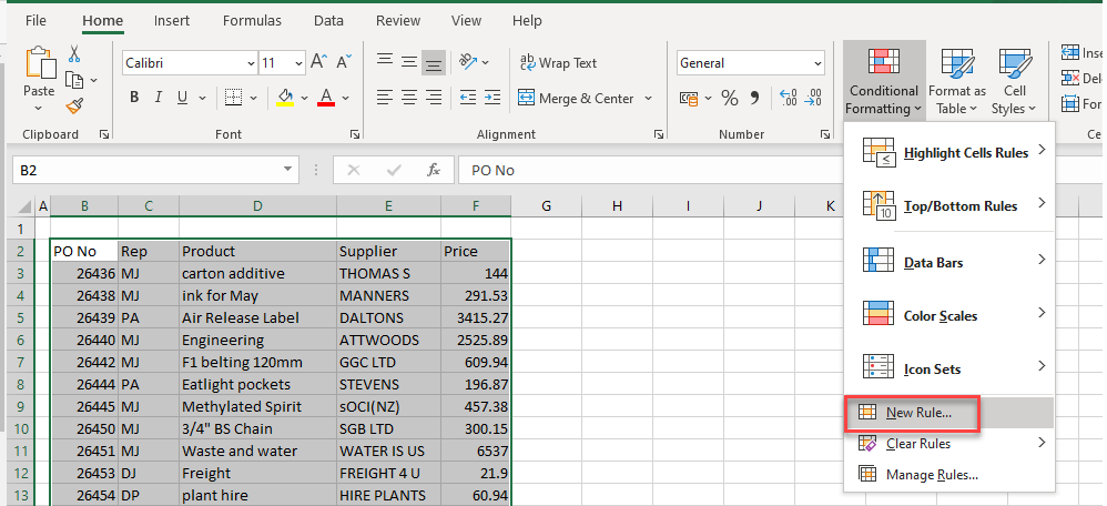
- Highlight the cells whose rows you wish to select. In the Ribbon, go to Home > Cells >Conditional Formatting.
- Select (1) Use a formula to determine which cells to format and then (2) enter the formula:
=MOD(ROW(B3),2)=0Then (3) click on Format…
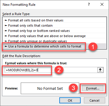
- The ROW Function returns the row number of the cell.
- The MOD Function, here, tests whether a number is even or odd by returning the remainder of the ROW formula divided by 2.
- In the Fill tab, select the color to format each alternate row, and click OK.
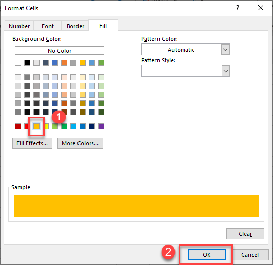
- Click OK again to apply the formatting to your worksheet.
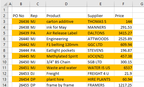
- As with Format as a Table, you can now Filter by Color to select every alternate row.
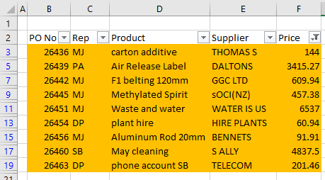
All the rows with the yellow cells are shown.
Select Every Other Row in Google Sheets
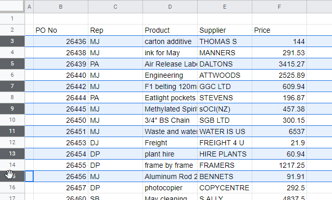
As with Excel, you can select every other row in a Google Sheet by selecting the first row and then holding down the CTRL key and selecting each alternate row thereafter.
You can also use conditional formatting and filtering to select every other row.
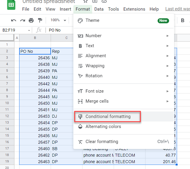
- Highlight the cells whose rows you wish to select. In the Menu, select Format > Conditional Formatting.
- Select (1) Custom formula is from the Format cells if… list and then (2) type in the following formula:
=MOD(ROW(B3),2)=0Then (3) select the color you wish every other row in the selection to be formatted with.
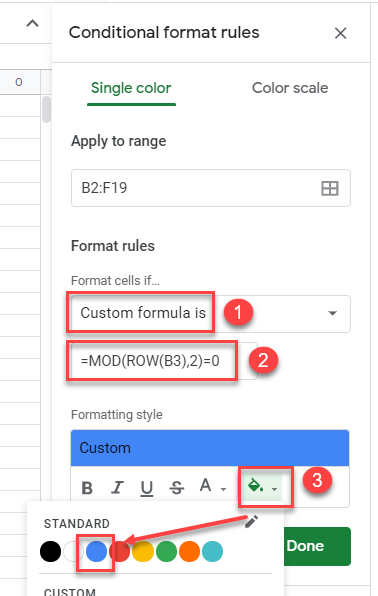
- Click Done to format the sheet.
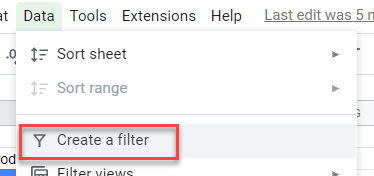
- Then create a filter to filter the rows by color.
In the Menu, select Data > Create a filter.
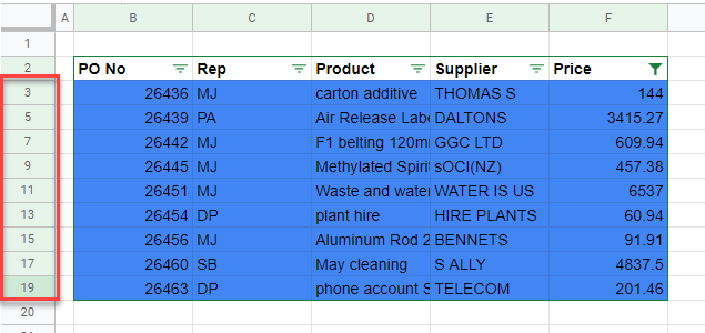
- In the filter drop-down list at the top of one of the columns, select Filter by Color > Fill Color and then select which color to filter on.

Every other row is now shown.
See also: How to Display Data With Banded Rows