How to Split a Cell Diagonally in Excel
This tutorial shows how to divide cells diagonally in Excel.
Insert a Shape
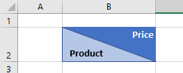
You can divide a single cell diagonally in Excel by inserting a right triangle shape into the cell.
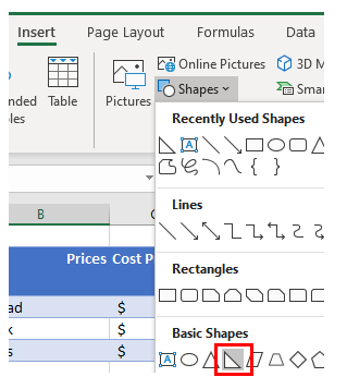
- In the Ribbon, choose Insert > Shapes > Right Triangle.
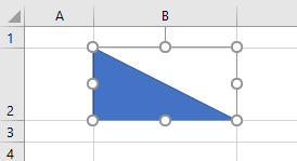
- Hold down the ALT key on the keyboard and draw the triangle in the cell.
Holding ALT makes the triangle snap to cell boundaries.
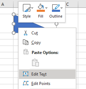
- Right-click the triangle and choose Edit Text.
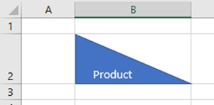
- Enter the desired text. If the text does not fit properly, widen the column and the triangle should automatically adjust to the width of the column.
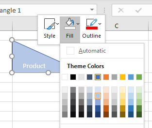
- Right-click on the triangle and then select Fill. Choose from Theme Colors to change the background color.
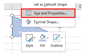
- Right-click the triangle and choose Size and Properties.
- To change the color of the text in the triangle, choose Home > Font > Font Color in the Ribbon.
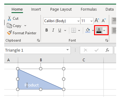
Tip: You can also change the fill of the triangle by clicking Home > Font > Fill Color.
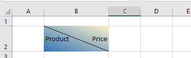
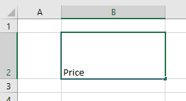
- To type the second half of the cell, click the cell (outside the triangle) and type the text you want.
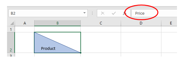
- Press ENTER, and the text disappears behind the triangle.
- In the Ribbon, select Home > Alignment and change the vertical alignment of the text to top and the horizontal alignment to right.
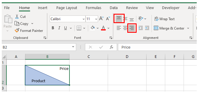
- Format the cell with the desired background and text color.
Insert Diagonal Frame
Alternatively, you can insert a diagonal frame into the cell to split the text.
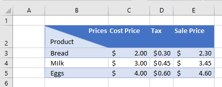
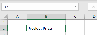
- Select the cell to be split and enter the desired text with a space between the words.
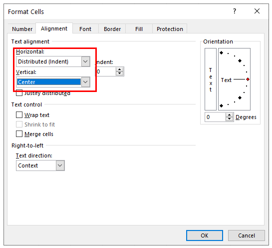
- In the Ribbon, choose Home > Font > Format Cells, and then choose the Alignment tab to change the alignment of the cell. Change the horizontal alignment to Distributed (Indent) and the vertical alignment to Center.
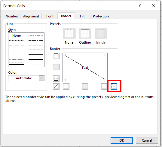
- Select the Borders tab and click the appropriate border to split the cell diagonally.
- If you want to change the color of the cell, click the Fill tab, and then click Fill Effects.
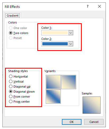
- Click OK to apply the effect.