How to Filter Pivot Table Values in Excel

This tutorial demonstrates how to filter pivot table values in Excel.

 

 

In-built Filter Area in a Pivot Table

When you create a pivot table, the column headers in the data become the fields of the pivot table. You can drag these fields in the data down to various areas of the pivot table – one of which is the Filters area.

 

 

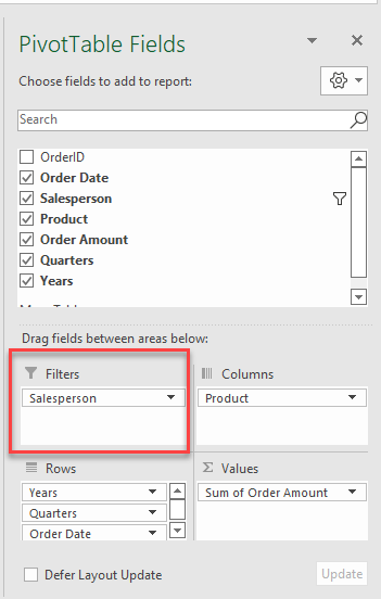
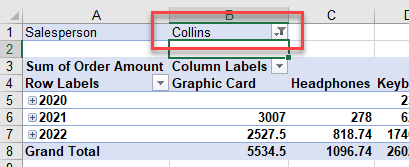
You can then filter the pivot table by this field. Select the drop-down filter and then select the item to filter one and finally select OK.

 

 

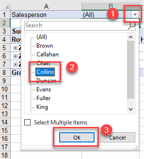
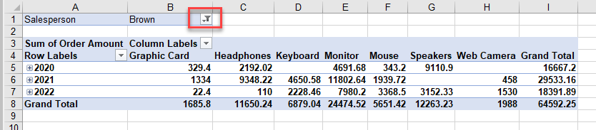
Your data is filtered accordingly.

 

 

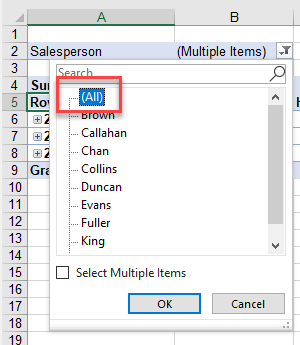
To clear the filter, click on the drop-down list, and then click on (All) and click OK.

 

 

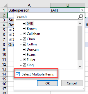
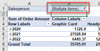
If you want to filter on multiple items, tick the Select Multiple Items check box.

 

 

Then, take the tick off the (All) check box and tick the items you wish to filter on. Finally, (3), click OK.

 

 

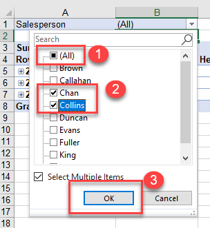
The filter indicates that you are filtering on multiple items.

 

 

To clear the filter, click on the drop-down list and then click on (All) once again and click OK.

Filtering by Row and Column Labels

You can also filter by the Row and Column Labels. Click on the drop down to the right of the Column Labels label and then remove the tick from (Select All) and tick the item you wish to filter on.

 

 

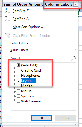
Click OK to filter the data.

 

 

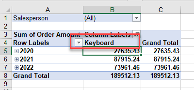
Similarly you can filter the Row Labels

 

Filter Pivot Table Values by Date

If you have dates in your pivot table, you can filter by these dates. This can be done in the Filter area, Row area or Column area.

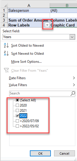
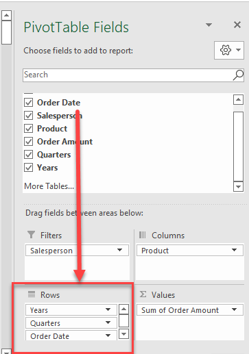
When a date is added to the Row or Column area, it is automatically broken down into 3 fields – Years, Quarters and the actual value of the date field itself. All 3 of these fields are then added to the Row or Column area.

 

 

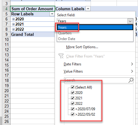
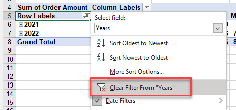
You can then click the Row Labels filter drop down, and then in the Select Field drop down, select the actual field to filter on.

 

 

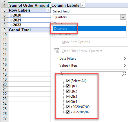
Amend the filter field to filter on Quarters instead of Years.

 

 

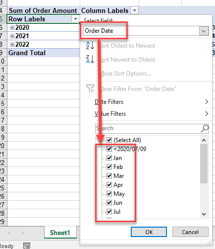
If you select the actual field to order on (e.g., Order Date), you’re then able to filter by Months.

 

 

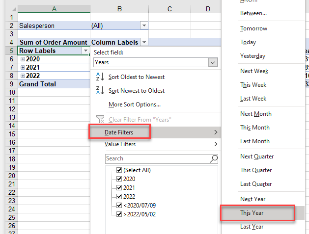
You can also select Date Filters from the menu, and then select the filter you need – for example, This Year.

 

 

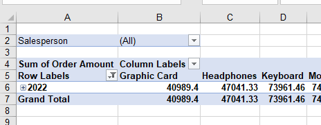
This immediately filters the data for this year only.

 

 

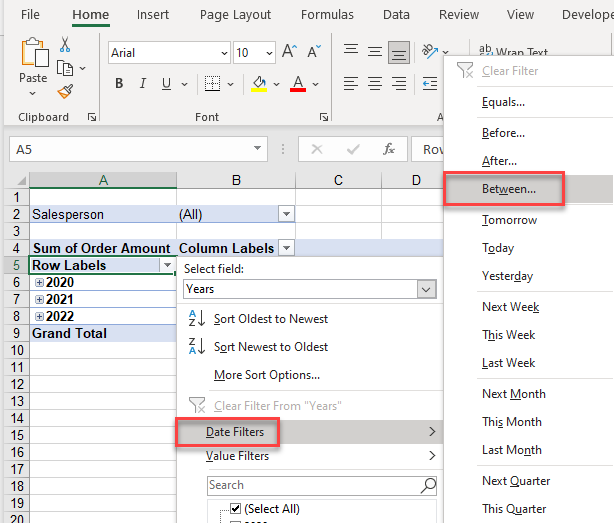
You can also be more specific and select the start and end dates to filter on.

In the drop-down list, select Date Filters > Between.

 

 

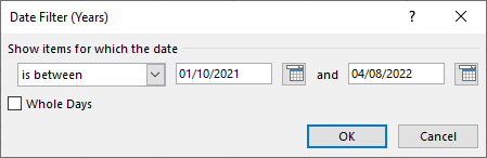
Then select the start and end dates to filter on and click OK.

 

 

Notice a small filter icon in the row labels drop-down box indicating that your data has a filter applied to it.

 

 

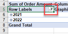
To clear the filter, click Clear Filter from “Years” in the drop-down menu.

 

 

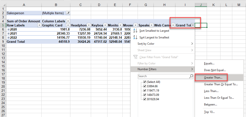
Create a Filter

The Values shown in a pivot table do not have a filter automatically in place for them.

To create a filter on these values, place your cursor to the right of the pivot table, and then, in the Ribbon, select Home > Editing > Filter.

 

 

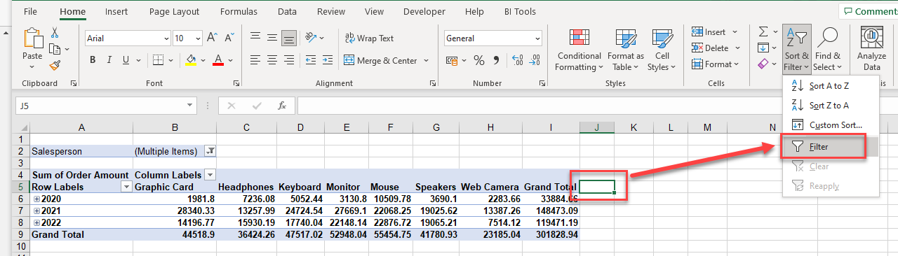
This will add a filter to the header of each of your column labels. You can then filter on the values accordingly. For example, you can select any of the individual values in the list, or you can select one of the Number filters such as values that are Greater Than a certain amount.